Foundational
Template matching
Template matching is a technique for recognizing which parts of an image match a template that represents a model image.
Clearly the template is smaller than the image to be analyzed.
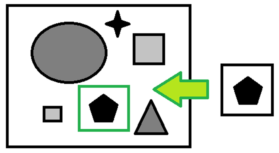
There are many techniques to do this, the main ones being:
- Comparing the pixel values of the template and image.
- One example is SAD (sum of absolute difference) which associates a new size matrix to the image, equivalent to:
- Number of rows = number of image rows - number of template rows
- Number of columns = number of image columns - number of template columns
The values of each element of the matrix will be:
Where r and c stand for the row and column coordinates and the sum is constructed on r’,c’ the template coordinates, therefore between 0 and the value of the template rows/columns. The closer this value is to zero the more likely the analysed portion will match the template. This approach is greatly affected by the absolute value of the pixel. The soundness of the search can be increased with a simple normalization based on the averages of the pixel values of the template and of the image.
- Comparison between template features and image features. One example is shape matching which compares the vectors of the gradients of the image outlines.
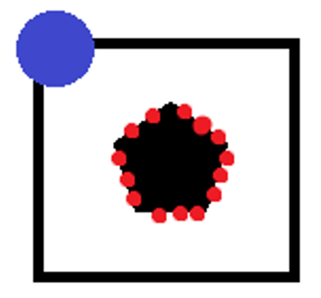
Some points of the outline (red dots) are extracted from the template, the positions of these points are saved with respect to a coordinate of reference (blue dot) which in our case has coordinate (0,0), the vectors of the gradients for each point of the template in question are saved.
The vectors of the gradients of the template and of the image are then compared, scrolling the coordinates of the reference point along the entire image. A matrix is associated with dimensionality equal to:
- Number of rows = number of image rows - number of template rows
- Number of columns = number of image columns - number of template columns
With values
With the sum constructed on the subset of the selected template points. Therefore, the gradient vector of point i of the image GI with coordinate (u,v)=(r,c)+(xi,yi) – where (r,c) is the new offset and (xi,yi) the relative position of the point to be analyzed with respect to the reference point in the template – is compared with the gradient of the point with coordinates (xi,yi) of the template GT.
Thanks to normalization, these values are always between -1 and 1. If the orientation of the gradient is irrelevant, but one is only concerned in its direction, the formula can be modified:
In this case, the values will still be between 0 and 1.
The closer the value is to 1, the more likely it is for the image to contain the required template.
The methods put forth above have the scale and rotation unchanged, but they can be modified to be adapted to this purpose.
Contour analysis
An image or a contour (binary image) can be analysed by moments.
A moment M under an order (p, q) is defined as follows:
With the double integral running over the whole domain of x and y (whole image or ROI).
As digital images represent a discrete subspace, we can replace the double integral with a double summation:
Simple moments:
- If we calculate M00 of the pixel intensity function I(x, y), we obtain the sum of the pixel values for monochrome images
- If we calculate M00 of the indicator function reporting the presence of non-zero pixels (unit value per pixel other than zero, otherwise null), we obtain the contour area.
- The image centroid coordinates can be calculated as follows:
The central moments (referring to the centroid coordinates) can be calculated based on the previous moments
Which have the property of being invariant with respect to translations (the centroid coordinates are based on M moments).
Invariance can be extended:
- to scale variation by calculating normalized moments
- based on scale variation and rotation through Hu moments.
Clearly, the latter are the most widely used.
Hu moments are a concise way of describing complex images.
Kernel
The kernel is a small mask used to apply filters to an image. These masks have the shape of a square matrix, which is why they are also called convolution matrices.
Let’s consider matrix A, which represents the matrix containing the grey values of all the pixels in the original image, and matrix B representing the kernel matrix. Now let’s superimpose matrix B to matrix A, so that the centre of matrix B corresponds to the pixel of matrix A to be processed.
The value of the target image (matrix C) is calculated as the sum of all the elements of the matrix resulting from the Hadamard product between matrices A and B.
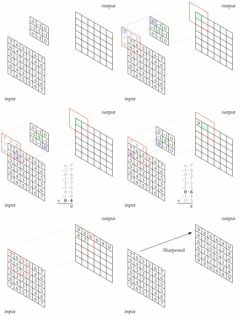
Example:
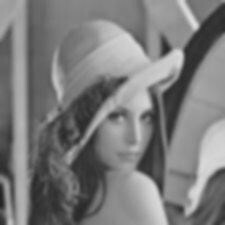
By applying a 3x3 blur filter
1/9 |
1/9 |
1/9 |
1/9 |
1/9 |
1/9 |
1/9 |
1/9 |
1/9 |
we can obtain this result:

Particularly useful kernels are derivative filters. Let’s analyse two Sobel filters:
1 |
0 |
-1 |
2 |
0 |
-2 |
1 |
0 |
-1 |
1 |
2 |
1 |
0 |
0 |
0 |
-1 |
-2 |
-1 |
These two filters represent, respectively, the derivatives (gradients) along abscissas Gx and along ordinates Gy of the image. If one calculates an additional matrix that represents the gradient module:

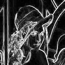
Clearly, this process represents the preliminary step to extract the edges of the image.
Edge detection
The edges are areas of the image where the intensity of the pixels suddenly varies.
As a first step, let’s analyse the plot profile of the following image:

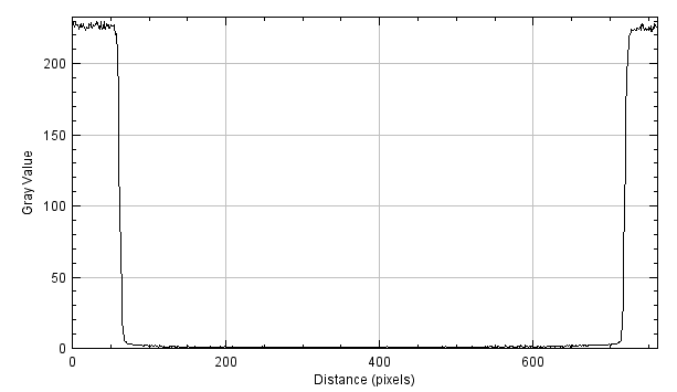
By applying a derivative filter (e.g. Sobel along x), we obtain the following graph (as an absolute value):
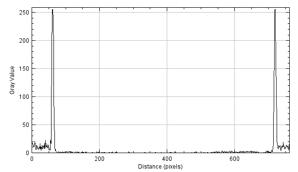
The edges are conventionally identified as the local maximum points of this graph. Sometimes, if there is the need to calculate the edge in subpixels, a fit of the neighborhood of the maximum values is carried out with a parabola.
In general, to calculate edges you need:
- A derivative filter
- An instrument to identify the maximum values in the calculated image.
Let’s take a look in detail of the procedure starting from the following image:
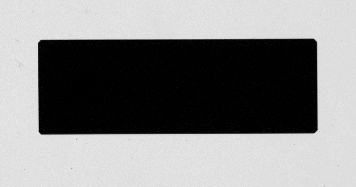
If we apply Sobel we obtain:

Let’s analyse in detail the previous image. To identify local maximum values we use an algorithm called Canny.
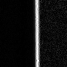
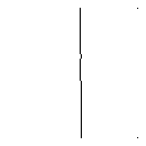
As well as suppressing points that do not represent a local maximum value, the algorithm carries out a procedure called thresholding with hysteresis. Two thresholds are defined, a low and a high one, which at each point are compared with the gradient. A point with a gradient above the upper threshold will certainly be accepted, a point with a gradient below the lower threshold will be rejected. A point with a gradient between the two thresholds is accepted only if the first neighbouring point has already been accepted.
The presence of two thresholds (hence the reference to the hysteresis) is justified by the fact that it is practically impossible to find a single brightness gradient value to determine whether a point belongs or does not belong to an edge. At the end of this step a binary image is obtained, where each pixel is marked as belonging or not belonging to an edge.
The segmentation of an image is the process of dividing it into significant regions in order to highlight some parts and make them easier to analyse.
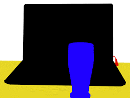
A simple segmentation method is so-called Thresholding, where the image is divided based on pixel intensity.
Example:

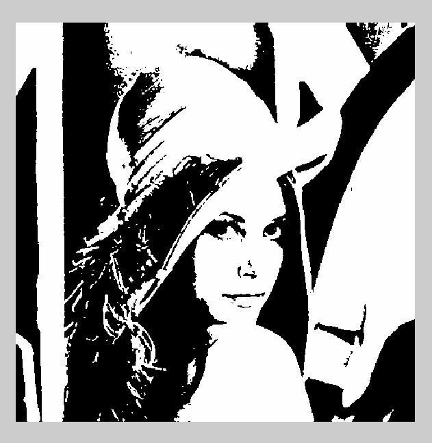
The pixel of the resulting image is a (set) non-zero value only if the corresponding pixel of the starting image is above a certain threshold (to be selected)
Blob analysis
Blobs are groups of pixels in an image with some shared properties (e.g. greyscale value).
Any blob analysis starts by identifying these areas in the image by using tools called blob detectors.
How does a blob detector work?
- Turn the image into a set of binary images. If the image is in greyscale, the task is a simple thresholding on the image, while if the image is in colour, each channel will be thresholded independently. In the set of images, each one of them represents a thresholding operation at a different threshold.
- The connected areas are identified in each binary image of the set.
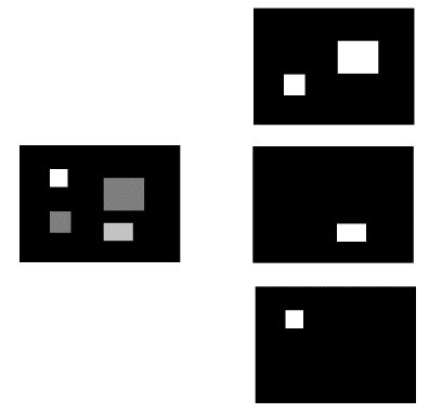
- The blob coordinates are identified and grouped by threshold ranges.
Once the blobs have been identified, they can be analysed by calculating scalars such as:
- Area
- Perimeter
- Convexity
- Circularity
- Compactness
Shape fitting
When the outlines have been extracted, the geometrical primitives must be extracted from them.
The main ones are:
- Fitting lines
- Fitting circles
- Fitting ellipses
Linear and circular fitting
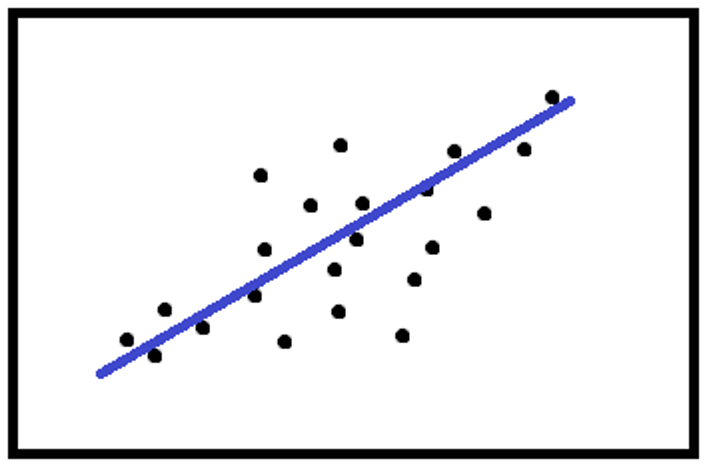
In both cases, the most commonly used algorithm is minimization, with the least-squares of the distance of the data points from the line or from the circumference.
The calculation can be made with the same weight for each point
Or, the weight can depend on the distance between the points and the calculated line or circumference.
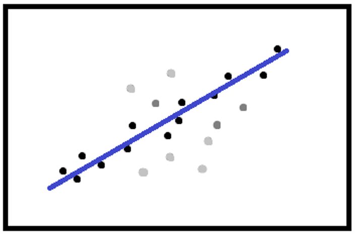
There are many functions to calculate the weights, the main ones being:
- Huber
Where c is a value chosen by the user, d is the distance of the point of the primitive.
- Tukey
normally the value of c is set at twice the standard deviation of the distribution of the distances.
The difference between Huber’s and Tukey’s functions is that in the former, the weights have a unit value for d less than or equal to c, and the function never reaches zero, while in Tukey the weights always have different values for d less than or equal to c, and zero elsewhere.
Sometimes, the RANSAC algorithm is used to build a robust fit.
Elliptical fitting
The most commonly used algorithm is an algebraic method, called the Fitzgibbon method.
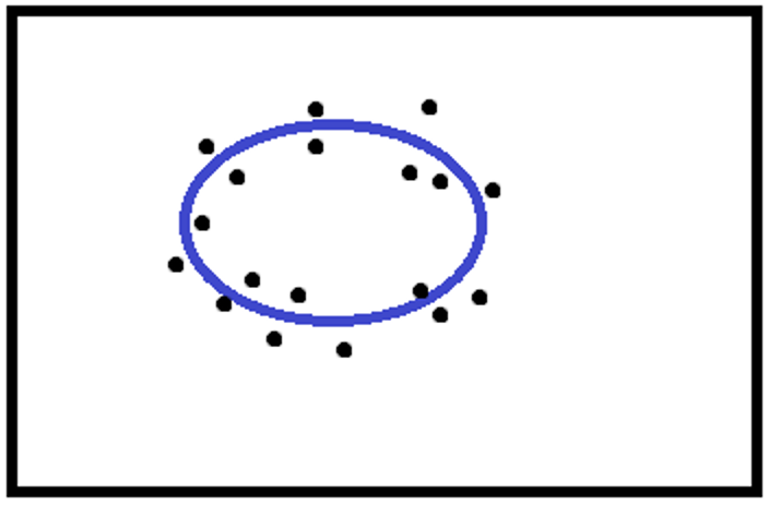
The elliptical fitting poses a few problems if the points only belong to certain parts of the ellipse
Examples:
- Correct fit
- Ambiguous fit
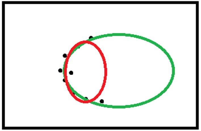
The algorithm outcome may be the red ellipse, though the green ellipse is the correct one.
Autofocus
To calculate the right focus for an image, we will use the Laplacian derivative filter.
-1 |
-1 |
-1 |
-1 |
8 |
-1 |
-1 |
-1 |
-1 |
By applying this filter to the image we will obtain the following result. As this is a derivative filter, the intensity of the pixels in the target image will appear greater if the neighboring pixels in the starting image have very differing intensity levels. Indeed, one can see that in the target image there is a greater intensity near the edges.

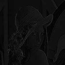
The last step consists in analyzing the histogram of the image (pixel intensity distribution in the image).
Let’s consider two cases: an image and the same image that a blur filter has been applied to (to simulate a poor focus). The histograms of the image on which the Laplacian filters have been applied are as follows:

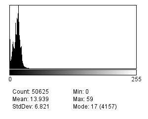

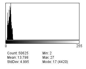
If one calculates the deviation of the two histograms, the unblurred image will have a poorer distribution due to the presence of higher maximum values (more marked edges).
How can you assess the focus quality?
- Collect a set of images (image set A).
- Apply the Laplacian operator to each image (image set B).
- Assess the histograms of image set B
- Identify the histogram with the highest standard deviation.
- The image of set A, corresponding to the identified histogram, is the image with the best focus.
Limits of this approach:
It is based on the comparison between histograms, so this approach is valid only if both images have the same subject.
